Calculating and visualizing standard deviations in two dimensions

The spread of points in one dimension is easy to calculate and to visualize, but the spread of points in two (or more) dimensions is less simple. Instead of familiar error bars, standard deviational ellipses (SDEs) represent the standard deviation along both axes simultaneously. The result is similar to a contour line that traces the edge of one standard deviation, as on a topographic map or an isochore map. The calculation of a standard deviational ellipse can be tricky, because the axes along which the ellipse falls may be rotated from the original source axes.

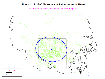
Figure 4.14 from CrimeStat III -- points representing locations of car thefts in Baltimore, with an ellipse indicating the highest density of thefts.

The standard deviational ellipse algorithm is described here and here, and it was implemented in aspace, an R library for geographic visualization work developed by Randy Bui, Ron N. Buliung, and Tarmo K. Remmel. The SDEs are calculated by calc_sde and are visualized by plot_sde. (The people who are most interested in multi-dimensional standard deviations seem to be geographers visualizing point data; an example of visualizing auto theft in Baltimore appears at right.)

The aspace SDE implementation is a very useful implementation. I’m going to talk about implementing three extensions to it:

Giving better example code for how to use the package.
Fixing a bug in which the ellipse is often incorrectly rotated by 90 degrees. [This has been fixed by the authors in aspace 3.2, following contact from me.]
Adding a feature that shows more than one standard deviations.

This post addresses each in turn.

More Thorough Example Usage Code for `aspace::plot_sde`

plot_sde doesn’t take the result of calc_sde as a parameter, and its documentation doesn’t indicate how R knows which SDE to draw. To draw an SDE, run plot_sde immediately after calc_sde. R uses an implicit object hidden from the user to pass data. A better usage example is:

# Example aspace::calc_sde and aspace::plot_sde Code
library(aspace)
# Create the data and rotate it
x = rnorm(100, mean = 10, sd=2)
y = rnorm(100, mean = 10, sd=4)
t = -pi/4 # Illustrates normal case (rotated to right from vertical)
#t = pi/4 # Illustrates the bug described below (rotated to left from vertical)
transmat = matrix(c(cos(t),-sin(t),sin(t),cos(t)),nrow=2,byrow=TRUE)
pts = t(transmat %*% t(cbind(x,y)))
# Create the plot but don't show the markers
plot(pts, xlab="", ylab="", asp=1, axes=FALSE, main="Sample Data", type="n")
# Calculate and plot the first standard deviational ellipse on the existing plot
calc_sde(id=1,points=pts);
plot_sde(plotnew=FALSE, plotcentre=FALSE, centre.col="red",
         centre.pch="1", sde.col="red",sde.lwd=1,titletxt="",
		 plotpoints=TRUE,points.col="black")
# Label the centroid, explicitly using the hidden r.SDE object that was used in plot_sde
text(r.SDE$CENTRE.x, r.SDE$CENTRE.y, "+", col="red")

The above code will plot the data without axes, layering the SDE ellipse on top of a plot that does not display data markers (as illustrated at below right).

Correct Visualization Regardless of Major Axis

Original ellipse is off by 90 degrees from the scattered points; improved ellipse is not.

14 August 2012: This has been fixed by the authors in aspace 3.2 following contact from me.

The aspace 3.0 calc_sde code (accessible by typing the function name without parentheses at the R prompt) includes the lines:

if (tantheta < 0) {
	theta <- 90 - atan_d(abs(tantheta))
} else {
	theta <- atan_d(tantheta)
}

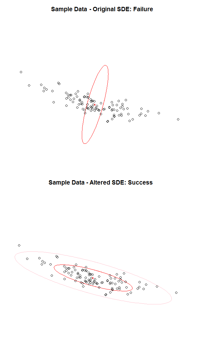
This code seems to aim to ensure that theta is a positive number — but the first line doesn’t ensure that. Instead it causes negative rotations to end up at 90 degrees to where they should be (as in the illustration at right). Instead that first if-clause could be:

if (tantheta < 0) {
	theta <- 180 - atan_d(abs(tantheta))
} else {
	theta <- atan_d(tantheta)
}

This code is one of multiple options that fixes the off-by-90-degrees issue.

Display of Multiple Standard Deviations

The aspace 3.0 calc_sde code only will only trace an ellipse of one standard deviation in each direction. To change this, add a multiplicative factor to sigmax and sigmay immediately before (or immediately after) the following lines:

if (sigmax > sigmay) {
	Major <- "SigmaX"
	Minor <- "SigmaY"
}
else {
	Major <- "SigmaY"
	Minor <- "SigmaX"
}

For instance, to calculate (and therefore plot) two standard deviations around the centroid, add in the lines:

sigmax=sigmax*2
sigmay=sigmay*2

These lines double the length of the single-standard-deviation major and minor axes.

—
Updated 2012-08-14.

Pamela Toman